The Graphing Commands: Plotting Graphs with Scaling and Labeling
You may often want to plot a horizontal or vertical bar graph or other kinds of graphs to display relationships. There exists a group of TUTOR commands which collectively make it very easy to produce such displays. In particular, scaling of your variables to screen coordinates is automatic, as is the numerical labeling of the axes, with tick marks along the axes. Figure 9-5 shows some examples. Suppose you want a graph to occupy the lower half of the screen. The horizontal x-axis should run from zero to ten and the vertical y-axis from zero to two. Both axes should be labeled appropriately. These statements will make the display shown in Figure 9-6.
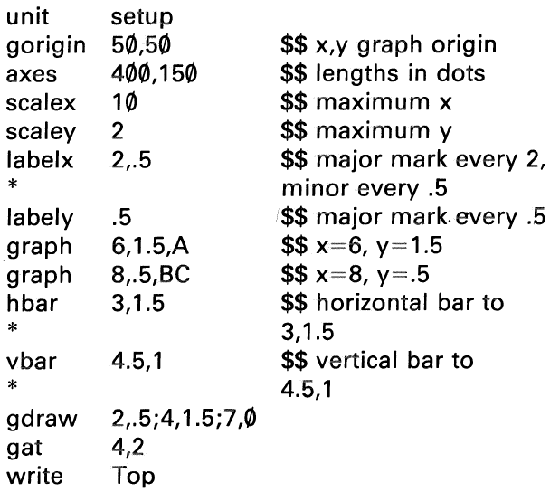
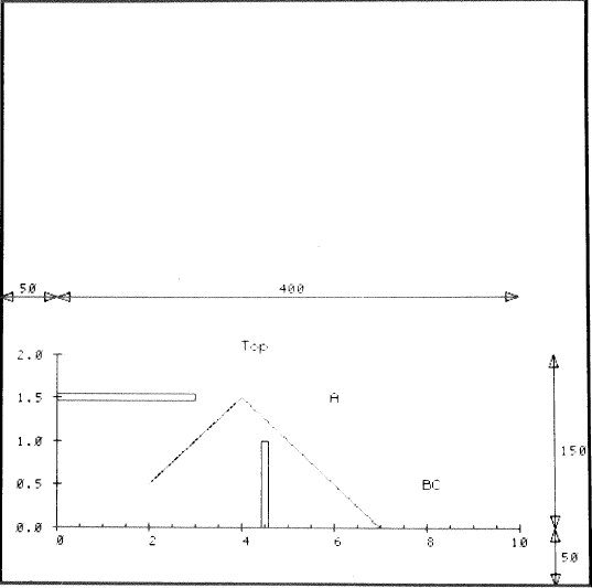
After specifying -gorigin- and -axes- in terms of fine-grid screen coordinates, the -scalex- and -scaley- commands associate scale values with the end points of the axes. These scale values determine how (x,y) coordinate positions given in later statements will be scaled to screen coordinates. The -labelx- and -labely- commands cause numerical labels and tick marks to appear. The statement “graph 6,1.5,A” plots an A at x=6, y=1.5 in scaled coordinates. The -hbar- and -vbar- commands draw horizontal and vertical bars to the specified scaled points. The -gdraw- command is like -draw-, except points are specified in terms of scaled quantities. The -at- command is like -at- but uses scaled quantities.
Read the example over and try to identify in the picture what part of the display results from each statement. (Keep in mind that each number in the tags of these statements could have been a complicated mathematical expression.)
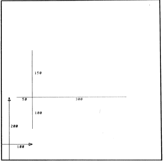
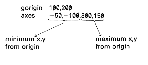
The -markx- and -marky- commands are similar to -labelx- and -labely- but merely display tick marks without writing numerical labels. The -axes- command has an alternative form which allows for axes in the negative directions. (See Figure 9-7.)
Although the commands were originally designed to make it easy to draw graphs, the automatic scaling features make these commands useful in many situations. Note, in particular, that you can move complicated displays around on the screen merely by changing the -gorigin- statement.
Additional graphing commands include -gvector- for drawing a line with an arrowhead at one end, -polar- for polar coordinates, and -lsealexand -lscaley- for logarithmic scales. The -bounds- command has the same effect as -axes- in establishing lengths, but no axes are drawn on the screen (a later blank -axes- command will display the axes). The -gboxcommand is used to draw rectangular boxes easily. The -gcircle- command draws circles or, if the x- and y-scales are different, -gcircle- will draw an ellipse.
Functions can be plotted very easily with the -funct- command. For example, “funct 5sin(2w),w⇐1,5,.02” will plot the function “5sin(2w)” by evaluating this function for values of w running from 1 to 5 in steps of .02. Note the similarity to the form of the iterative -do- statement. If there was an earlier “delta .02” statement, we can leave off the increment and simply write “funct 5sin(2w),w⇐1,5”. If, in addition, we want the function to be plotted all the way from the left edge of the established axes to the right edge, we simply write “funct 5sin(2w),w”.